How Markets Work
Cheat sheet
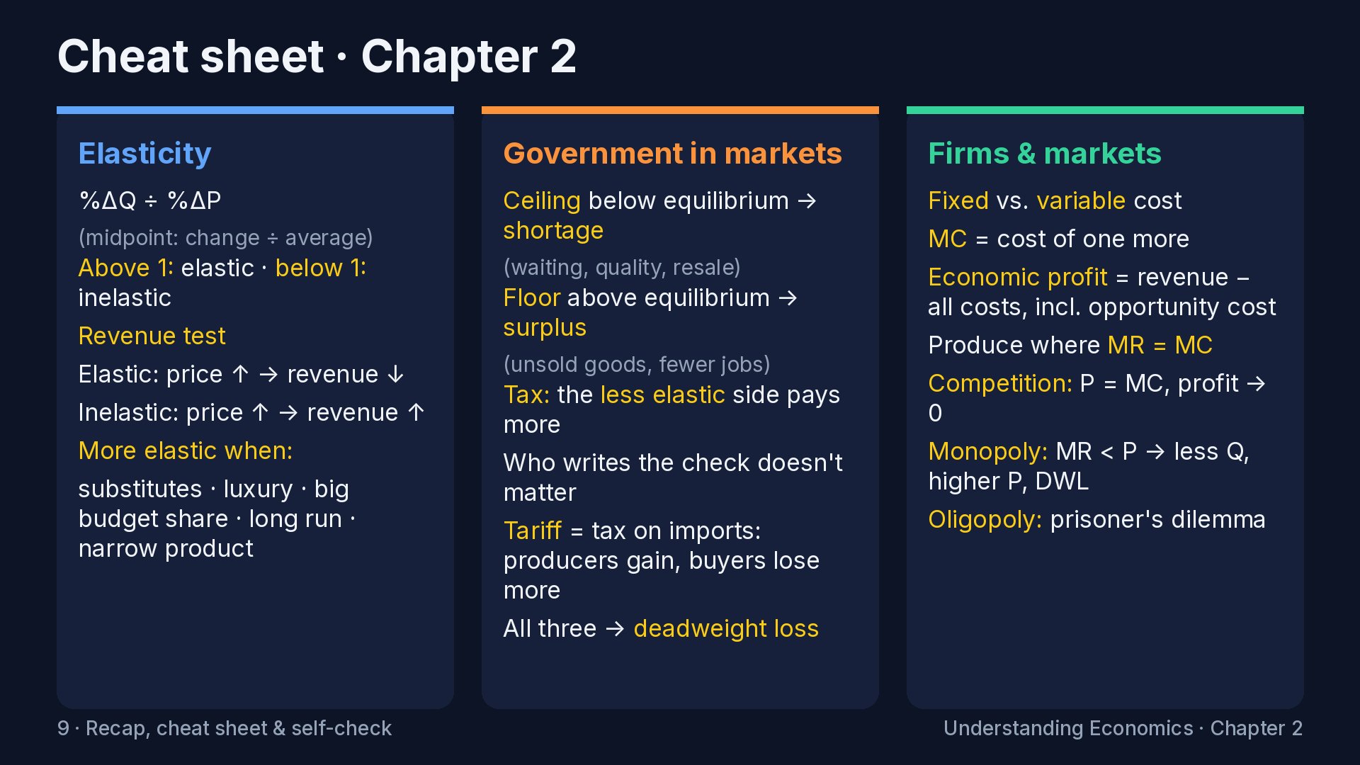
Transcript
The airfare puzzle
Welcome to Chapter 2 of Understanding Economics. In this chapter, we'll measure how strongly people react to a price change, and who really wins when a market trades. Then we'll look at what happens when governments cap prices or add taxes, and why a monopoly behaves so differently from a competitive market. Here's a puzzle. You look up a flight, and a seat costs eighty-nine dollars. A week later, the same seat on the same plane costs four hundred. Those are illustrative numbers, but you've probably seen something like it. Nothing about the seat changed. So why did the price? By the end of this chapter, you'll be able to explain it. A quick recap of Chapter 1. Demand slopes down, supply slopes up, and the price settles where the two curves cross. Below that price you get a shortage, and above it, a surplus. Today we put that machine to work, starting with one question: when a price changes, how much do people actually react?
Elasticity
Elasticity. This is one of the most useful ideas in all of economics, so we'll take our time with it. From Chapter 1, you know the law of demand. When the price goes up, people buy less. That tells us the direction. But it doesn't tell us how much less. And that's often the question that matters most. If a coffee shop raises its price by ten percent, does it lose a few customers, or half of them? If gas goes up fifty cents, do people drive a little less, or a lot less? Economists have a name for how strongly buyers react to a price change. It's called elasticity. Here's the definition. The price elasticity of demand is the percentage change in the quantity people buy, divided by the percentage change in the price. On top: by what percent did the amount people buy change? On the bottom: by what percent did the price change? We use percentages so we can compare anything to anything. Cups of coffee and gallons of gas and concert tickets are measured in totally different units, but a percent is a percent. One more thing: demand slopes down, so this number technically comes out negative. Economists usually just drop the minus sign and talk about the size. That's what we'll do. If the number is bigger than one, demand is elastic. The quantity changes by a bigger percent than the price did. Raise the price ten percent, and sales drop by more than ten percent. Buyers are sensitive. If the number is less than one, demand is inelastic. The quantity changes by a smaller percent than the price. Raise the price ten percent, and sales drop by less than ten percent. Buyers mostly keep buying. And if it's exactly one, it's called unit elastic. The two percentages match. It's the dividing line between the other two. Let's work one. These are illustrative numbers. A streaming service raises its monthly price from ten dollars to twelve. Its subscribers drop from one thousand to seven hundred. First, the percent change in price. Here's one small trick. If you go from ten to twelve, that's a twenty percent increase. But if you go back from twelve to ten, that's only about a seventeen percent decrease. Same two prices, two different answers. To avoid that, economists use the midpoint method: divide the change by the average of the two values. The price changed by two dollars, the average price is eleven, so the change is about eighteen percent. Now the quantity. Subscribers fell by three hundred. The average of one thousand and seven hundred is eight hundred and fifty. Three hundred divided by eight hundred fifty is about thirty-five percent. So the elasticity is thirty-five divided by eighteen, which is about one point nine. That's bigger than one, so demand for this service is elastic. A modest price increase drove away a lot of subscribers. That makes sense. There are plenty of other streaming services to switch to. Here's what elasticity looks like on a graph. Take a steep demand curve. Start at a price of five dollars. Now raise the price to six. The quantity barely moves. That's inelastic demand. Think of gasoline this week. Most people still have to drive to work, so even if the price jumps, they keep buying almost the same amount. Now a flat demand curve, through the same starting point. Same one-dollar price increase, and the quantity collapses. That's elastic demand. Think of one particular brand of coffee in a store full of other brands. Raise its price, and shoppers simply grab the one next to it. So a quick rule of thumb: the flatter the demand curve, the more elastic it is. The steeper, the more inelastic. One caution: on a straight-line demand curve, elasticity actually changes as you move along it. It's more elastic at high prices and less elastic at low prices. So the slope is a good visual hint, but elasticity is really about percentages. There are two extreme cases worth knowing. Perfectly inelastic demand is a vertical line. The quantity doesn't change at all, whatever the price. Nothing is perfectly inelastic in real life, but a life-saving medicine with no substitute comes close. Perfectly elastic demand is a flat, horizontal line. Raise your price even a penny and your sales go to zero. A farmer selling wheat that's identical to every other farmer's wheat is close to this. If they ask for more than the market price, buyers just buy from someone else. Hold on to that one. It'll come back at the end of the chapter, when we talk about competition.
Elasticity & revenue (the airfare answer)
Now, why do businesses care so much about elasticity? Because of revenue. Total revenue is just the price times the quantity sold. On a graph, that's this rectangle: the price is the height, the quantity is the width. Now raise the price. Two things happen. You earn more on every unit you still sell. That's this yellow strip on top. But you also lose the sales that disappear. That's the red strip on the side. So does revenue go up or down? It depends on which strip is bigger. And that's what elasticity tells you. This is called the total revenue test. If demand is elastic, raising the price lowers revenue, because the lost sales outweigh the higher price. Our streaming service shows it. Revenue went from ten dollars times one thousand, which is ten thousand dollars, to twelve dollars times seven hundred, which is eight thousand four hundred. The price went up, and revenue went down. With elastic demand, cutting the price is what raises revenue. If demand is inelastic, it's the opposite. Raising the price raises revenue, because buyers mostly keep buying. Picture a gas station whose price goes up about eighteen percent while the gallons it sells drop only about five percent. Revenue goes up. That's also why a bad harvest can actually raise farmers' total revenue: food demand is inelastic, so prices jump by more than the quantity falls. And in the unit elastic case, the two effects cancel out, and revenue doesn't change. This test is a big part of how businesses think about pricing. And it's why the same company may run discounts on some products and quietly raise prices on others. So what makes demand elastic or inelastic? Five things. The biggest one is substitutes. The more alternatives people have, the more elastic demand is. One airline's flight on a busy route has lots of substitutes. Tap water at home has very few. Second, necessity versus luxury. Necessities, like basic groceries, electricity, and medicine, tend to be inelastic. You buy them anyway. Luxuries, like a cruise or a designer handbag, are elastic. It's easy to skip them. Third, the share of your budget. If salt doubles in price, you probably won't even notice. If your car payment doubles, you will. The bigger the slice of your budget, the more elastic. Fourth, time. In the short run, people are stuck. When gas prices jump, you still have the same car and the same commute. But give it a few years, and people buy more efficient cars, move closer to work, or take the train. So demand is more elastic in the long run than in the short run. And fifth, how narrowly you define the product. Demand for food overall is very inelastic. Demand for one brand of cereal is very elastic. Same aisle, completely different behavior. Time for the first pause and predict. An airline raises fares by ten percent on one route. Who reacts more strongly: people booking a vacation, or business travelers who need to fly tomorrow? And for which group does the airline's revenue go up? Pause the video, think it through, and then press play. Here's the answer. Vacation travelers are the elastic group. They can pick different dates, a different destination, or just drive. So a higher fare drives a lot of them away. Business travelers on a last-minute trip are inelastic. They have to be there, and soon. So for business travelers, the higher fare raises the airline's revenue. Hold on to that answer. It's half of our puzzle. One more quick one. Elasticity works on the supply side too. The price elasticity of supply asks: when the price rises, how much more do sellers produce? The biggest factor, again, is time. Right after a price jump, sellers can't do much. Given time, they can hire, build, and expand. So supply is more elastic in the long run. The other factor is spare capacity. A T-shirt printer that gets a rush of orders can just add a shift. Its supply is elastic. But a stadium can't add seats for tonight's concert. Its supply is nearly fixed, a vertical line. That's why, when demand for a hot concert spikes, nearly all the adjustment shows up in the price, and resale tickets go sky high. Now we can solve the puzzle from the start of the chapter. Why can the same seat cost eighty-nine dollars one week and four hundred the next? Start with supply. A plane has a fixed number of seats. Like the stadium, its supply can't stretch, so changes in demand show up almost entirely in the price. Next, who's buying early? Mostly people with flexible plans, often vacationers. Their demand is elastic. They can pick another date, another destination, or not go at all. So the airline sets low fares to fill seats with them. And who's buying at the last minute? Mostly people who have to be somewhere, like business travelers or someone heading to a family emergency. Their demand is inelastic. A high fare doesn't stop them. So the airline charges each group close to what that group will bear. Economists call charging different prices for the same thing price discrimination. Airlines also raise fares as a flight fills up, because each remaining seat gets scarcer. Fixed supply plus different elasticities: that's the core of the puzzle. Real airline pricing adds more, like competition between airlines and fare rules, but this is the engine.
Surplus
Who actually gains from a market? Economists have a way to measure it, and we'll need it for everything that comes after: price controls, taxes, and monopoly. Start with buyers. Imagine four fans who want a concert ticket. These are illustrative numbers. The first fan would pay up to a hundred dollars. The second, up to eighty. The third, up to sixty. And the fourth, only forty. That top number is called willingness to pay: the most someone would pay before they'd rather walk away. It reflects two things: how much someone wants the ticket, and how much they're able to pay. The fourth fan might love the band just as much as the first, but be on a tighter budget. The ticket costs fifty dollars. The first fan would have paid a hundred, but only pays fifty, so they walk away fifty dollars better off. The second fan is thirty dollars better off. The third, ten dollars. That gap, between what you would have paid and what you actually paid, is called consumer surplus. Add it up: ninety dollars of value that buyers got for free, just because the market price was lower than what they were willing to pay. And the fourth fan? Willing to pay only forty, so they don't buy. No surplus. That's fine. The market served the people who valued the ticket at least as much as it cost. Now let's put this on a graph. Here's a coffee market with illustrative numbers. Demand and supply cross at five dollars a cup and five hundred cups a day. Every point on the demand curve is someone's willingness to pay. The people on the left would have paid a lot more than five dollars. So consumer surplus is the whole area below the demand curve and above the price. This blue triangle. Sellers get a surplus too. Every point on the supply curve is the lowest price a café would accept for that cup, basically what it costs them to make it. They get five dollars. The gap is producer surplus: the area above the supply curve and below the price. This orange triangle. And because they're triangles, you can measure them. The area of a triangle is one half times the base times the height. The base is five hundred cups. The height of the blue one is from five dollars up to nine, so four dollars. One half times five hundred times four is one thousand dollars a day. The orange triangle has the same size, so another thousand. Add them together and that's the total surplus. That's the total value this market creates every day: two thousand dollars. Here's the key insight. In a competitive market, the equilibrium quantity makes the total surplus as large as it can be. That comes with conditions: real competition, no side effects that the price leaves out, the externalities we'll meet in Chapter 3, and buyers and sellers who are reasonably well informed. When those hold, every cup that's worth more to a buyer than it costs to make gets made and sold. And no cup gets made that costs more than it's worth. Economists call that efficient. So if something pushes the quantity away from equilibrium, some trades that would have made both sides better off don't happen. That lost value doesn't go to anyone. It just disappears. It's called deadweight loss. Remember that phrase. We're about to see it three times in a row.
Price ceilings & floors
What happens when the government sets a price directly, either a maximum or a minimum? This is where supply and demand gets really practical, so we'll go slowly. There are two kinds. A price ceiling is a legal maximum. Sellers can't charge more than this. Think of a cap on rent increases, or a cap on what can be charged for essentials during an emergency. A price floor is a legal minimum. Buyers can't pay less than this. The best-known example is the minimum wage, which is a floor on the price of labor. Both are usually put in place with good intentions: to protect renters, or to raise the pay of low-wage workers. Here, we'll just look at what the supply and demand model predicts. Then we'll talk about where the real-world debate comes in. Here's a rental market with no rules. Demand from renters, supply from building owners, and rent settles at equilibrium. Now put a ceiling below the equilibrium rent. It's the red line. Owners can't legally charge more than that. Look at what happens. At that lower rent, more people want apartments: that's the quantity demanded, Q d. But owners offer fewer: that's Q s. The gap between them is a shortage. More people are looking than there are apartments available. This is the same shortage we saw in Chapter 1, except now it can't fix itself, because the price isn't allowed to rise. And because fewer apartments are rented than at equilibrium, we get deadweight loss. This red triangle is trades that would have helped both a renter and an owner, but don't happen. Now, to be fair to the policy: the renters who do have apartments pay less. Some surplus moves from owners to those renters, which is often the whole point. The model's warning is about everyone else, the people searching for a place that isn't there. One more thing. A ceiling only matters if it's below the equilibrium price. If the cap is set above where the market would settle anyway, it's called non-binding, and nothing changes. When the price isn't allowed to ration a scarce good, something else does the rationing. First, waiting. Lines, waitlists, and months of searching. Your time becomes part of the price. Second, quality can slip. If an owner can fill a unit no matter what, there's less pressure to maintain or improve it. Third, side deals. Extra fees, resale markets, or payments under the table. Concert tickets capped at face value are a great example. The price still finds a way up. It just shows up on the resale site. And fourth, luck and connections start to decide who gets the good, rather than who values it most. This is why most economists are skeptical of rent control as a long-run fix, even while many people support it for protecting existing tenants. Real policies come in many designs, so the size of these effects depends a lot on the details. But the direction comes straight out of the graph. Now the opposite: a price floor. Here's a labor market. The demand for labor comes from employers. The supply comes from people who want jobs. The price of labor is the wage. Put a minimum wage above the equilibrium wage. At that higher wage, more people want to work: Q s. But employers want to hire fewer: Q d. The gap is a surplus of labor. In the simple model, that surplus is unemployment: people who want a job at that wage but can't find one. It's the same logic as farm price supports, where a floor on a crop's price leaves unsold crops piled up. There's a deadweight loss triangle again. But notice the trade-off. The workers who keep their jobs earn more. So a floor helps some people and can hurt others. How big is the job loss in practice? This is one of the most studied questions in economics, and studies disagree, often depending on how high the minimum is compared to local wages. Real labor markets have extra features that this simple graph leaves out, and we'll look at some of them in Chapter 3. So treat this graph as the starting point for the debate, not the final word. Side by side: a ceiling only bites below equilibrium and creates a shortage, with waiting, falling quality and resale markets. A floor only bites above equilibrium and creates a surplus: unsold goods or fewer jobs. Both bring deadweight loss when the quantity traded falls below equilibrium.
Taxes & tariffs
Taxes. Who really pays a tax? The answer surprises most people, because it has almost nothing to do with who hands the money to the government. Here's a market with illustrative numbers. Before any tax, the price is five dollars, and five thousand units are sold. Now the government puts a two-dollar tax on each unit, and the law says sellers have to pay it. For a seller, that's just like a two-dollar increase in costs. So the supply curve shifts up by exactly two dollars. The new equilibrium is where demand crosses the new supply curve. Buyers now pay six dollars. That's one dollar more than before. Sellers collect six, send two to the government, and keep four. That's one dollar less than before. So even though the law said sellers pay the tax, buyers and sellers each ended up carrying one dollar of it. And sales fell from five thousand to three thousand seven hundred fifty. The government collects two dollars on each of three thousand seven hundred fifty units. That's seven thousand five hundred dollars. It's this yellow rectangle. And there's our red triangle again: deadweight loss. Twelve hundred fifty units that would have been worth trading no longer get traded. One half times twelve hundred fifty times two dollars is twelve hundred fifty dollars of value that simply disappears. That's the hidden cost of a tax, on top of the money collected. Now the same two-dollar tax, but this time demand is inelastic. Buyers have few alternatives. Think gasoline, or cigarettes. Shift supply up by two dollars, and look where it lands. Buyers now pay six fifty, a dollar fifty more. Sellers keep four fifty, only fifty cents less. Buyers carry three quarters of the tax. Economists call this tax incidence: who really bears the burden. And the rule of thumb is simple. The side that's less elastic, the side that has a harder time walking away, pays more of the tax. If it were supply that was inelastic instead, sellers would carry most of it. And here's the surprising part. It doesn't matter who the law says pays. Put the same tax on buyers instead of sellers, and in the model you end up with the same split. The person who writes the check to the government isn't necessarily the person who pays. A subsidy, by the way, works the same way in reverse: a payment per unit, shared between buyers and sellers by the same rule. Second pause and predict. A new fifty-cent tax per gallon is charged to gas stations. In the short run, drivers can't easily change how much they drive. Who ends up paying most of that fifty cents? Pause, and predict. The answer is drivers. In the short run, gas demand is inelastic, so the price at the pump rises by most of the fifty cents. The stations hand the money to the government, but drivers carry most of the burden. Over many years, as people switch cars and commutes, demand gets more elastic, and the split shifts somewhat. Now a short look at tariffs, because a tariff is just a tax on imports. Here's a market for bicycles, with illustrative numbers. If the country is open to trade, bikes sell at the world price, three hundred dollars. At that price, home producers make two thousand five hundred, but buyers want seven thousand five hundred. Imports fill the gap: five thousand bikes. Now add a one-hundred-dollar tariff on every imported bike. The price at home rises to four hundred. Home producers make more, three thousand seven hundred fifty. Buyers buy less, six thousand two hundred fifty. And imports shrink to two thousand five hundred. So who wins and who loses? Home producers win: they sell more, at a higher price. The government collects the tariff on every imported bike: this yellow rectangle. Buyers lose: they pay more and buy less, and their loss is bigger than the other two gains combined. The difference is the two red triangles, the deadweight loss. Supporters of tariffs usually point to other goals, like protecting particular industries or jobs, or national security. The model says that those goals come at a cost, and that most of the cost lands on buyers. We'll come back to trade in Chapter 6.
Costs & profit
Before we compare competition and monopoly, we need a quick look inside a business: its costs and its profit. We'll go fast here. Take a food truck. Some costs are fixed. They don't change with how many meals you sell. The truck lease, insurance, permits. Sell zero meals or five hundred, you pay the same. Other costs are variable. They rise with every meal: ingredients, packaging, fuel for the generator. Total cost is just fixed cost plus variable cost. Simple. But the most important cost for decisions is the next one. Marginal cost is the extra cost of making one more unit. Here's a bakery, with illustrative numbers. At zero loaves, it still pays two hundred dollars a day. That's the fixed cost. Going from zero to one hundred loaves raises total cost to three hundred, so each of those extra loaves cost a dollar. The next hundred cost eighty cents each, because the bakers get into a rhythm and the oven runs full. Then a dollar. Then a dollar sixty. Why does marginal cost eventually rise? Because the kitchen is the same size. Squeeze in more bakers, and they start bumping into each other and waiting for the oven. Each extra loaf gets harder to make. Economists call this diminishing marginal returns. And here's the rule a profit-seeking business follows, at least roughly, whether it knows it or not: keep producing as long as one more unit brings in more money than it costs to make. Stop where they're equal. In economics shorthand: marginal revenue equals marginal cost. Last idea in this part: two kinds of profit. Someone runs a café for a year, with illustrative numbers. Revenue is two hundred thousand dollars. Rent, coffee beans, and staff cost a hundred fifty thousand. That leaves fifty thousand. This is accounting profit, the number on the tax return. But remember opportunity cost from Chapter 1. To run this café, the owner quit a job that paid seventy thousand a year. That's a real cost too, even though no check was written. Subtract it, and economic profit is minus twenty thousand. The café is profitable on paper, but the owner would be twenty thousand dollars better off back at the old job. Economists count all costs, including what you gave up. When economic profit is exactly zero, you're earning just enough to stay. That's called normal profit. Hold onto that. It's the key to what happens under competition.
Competition vs. monopoly
The last big one: competition versus monopoly. Why does the number of sellers in a market change the price you pay? Markets sit on a spectrum. At one end is perfect competition. Very many sellers, all selling the identical product. Think of farmers growing wheat. Next, monopolistic competition. Many sellers, but each product is a bit different. Coffee shops and restaurants. Each one has a small amount of pricing power because of its location or its menu, but plenty of rivals. Then oligopoly: a few big sellers. Airlines on a route, phone carriers, the major streaming services. Each one has to watch what the others do. And at the far end, monopoly. One seller, with no close substitute. A local water utility is the classic example. Let's look at the two ends first. In perfect competition, each seller is a price taker. Remember the perfectly elastic demand from earlier? That's what one wheat farmer faces. If they charge a penny above the market price, nobody buys from them. So they just take the market price. Using our rule, they produce until marginal revenue equals marginal cost. For a price taker, every extra unit sells at the market price, so marginal revenue is the price. That means they produce until price equals marginal cost. If farmers are earning economic profits, word gets around, and new farmers plant the crop. Supply shifts right and the price falls. If they're losing money, some leave, supply shifts left, and the price recovers. So in the long run, the price gets pushed down to the cost of production, and economic profit goes to zero. That's normal profit: just enough to stay in business. Great for buyers. And when the conditions from the surplus section hold, the market makes every unit worth making, so total surplus is as big as it can be. A monopoly is different. It isn't a price taker. It faces the whole market's demand curve. If it wants to sell more, it has to lower its price. Here are illustrative numbers. At ten dollars, it sells one unit. At nine, two. At eight, three, and so on. Now look at marginal revenue, the extra revenue from selling one more unit. Going from one unit to two, the price drops to nine. The monopoly gains nine dollars from the second sale, but loses a dollar on the first unit, which now also sells for nine. So marginal revenue is only eight. For the third unit, it's six. Because the monopoly has to cut the price on every unit it sells, marginal revenue is always below the price. Say each unit costs four dollars to make. The monopoly follows the same rule as everyone: produce until marginal revenue equals marginal cost. That's four units, at a price of seven dollars. A competitive market would keep going until price equals marginal cost, four dollars, and on this demand curve that's seven units. So the monopoly sells fewer units, at a higher price. Here's the same story on a graph. Demand slopes down. To keep it simple, marginal cost is flat: every unit costs the same to make. Now add marginal revenue. It starts at the same point as demand, but it falls twice as fast. It's below demand everywhere, for the reason we just saw: to sell one more, you have to cut the price on all of them. The monopoly picks the quantity where marginal revenue meets marginal cost. Then it goes straight up to the demand curve to find the highest price buyers will pay for that quantity. That's the monopoly price. Compare that to competition. A competitive market would produce where demand meets marginal cost. That's way out here, at a lower price and a much bigger quantity. The green rectangle is the monopoly's profit: the price minus cost on every unit it sells. And the red triangle is deadweight loss: units that buyers valued more than they cost to make, but that never get made. That's the core economic case against monopoly: a higher price and less output than buyers would happily pay for. Between those two ends sits oligopoly, a market with just a few big rivals. The key feature is that each firm's best move depends on what the others do. If one airline cuts fares on a route, the others notice by the afternoon. If the rivals all agreed to keep prices high, together they could earn almost what a monopoly would. That kind of agreement is called a cartel. But each one is tempted to undercut the others and grab more customers. So agreements like this tend to break apart. Economists study this tension with game theory: the study of decisions where your outcome depends on someone else's choice. The most famous example is called the prisoner's dilemma. Let's play it with two gas stations. Two gas stations sit across the street from each other. Each can charge a high price or a low price. These are illustrative daily profits, the North station's first and the South station's second. If both charge high, each earns a thousand dollars a day. That's the best outcome for the two of them together. But look at the North station's temptation. If South charges high and North charges low, North steals the customers and earns twelve hundred, while South drops to three hundred. Now think like the North station. If South charges high, North earns more by going low: twelve hundred instead of a thousand. If South charges low, North still does better going low: six hundred instead of three hundred. Either way, low is better for North. That's called a dominant strategy. And South faces exactly the same numbers. So both charge low, and each earns six hundred. Both would have been better off at a thousand, but neither could trust the other to stay high. That's the dilemma. It's bad news for the stations, and good news for drivers. In real life, rivals that compete every day sometimes learn to avoid price wars without ever talking. And if they explicitly agree to fix prices, in the United States and many other countries, that's against the law. So why do governments regulate monopolies? Because of everything we just saw: higher prices, less output, deadweight loss, and often less pressure to improve, since customers have nowhere else to go. The main tool is antitrust law. It's used to block mergers that would wipe out competition, and to ban things like price-fixing between rivals. Some industries are natural monopolies. It's cheapest for one company to run the whole network, like water pipes or power lines. Building a second set of pipes down every street would be a huge waste. So instead of breaking these companies up, governments usually regulate the prices they can charge. And sometimes the government creates a monopoly on purpose. A patent gives an inventor the sole right to sell an invention for a limited number of years. It's a trade-off: higher prices for a while, in exchange for the incentive to invent in the first place. That's the pattern you'll see all through economics. There are almost never free lunches, only trade-offs.
Recap, cheat sheet & self-check
Let's wrap up. Here's the whole chapter in about two minutes. Elasticity measures how strongly buyers react to a price change: the percent change in quantity, divided by the percent change in price. Substitutes, necessity, budget share, time, and how narrowly you define the product all decide it. The total revenue test: if demand is elastic, raising the price lowers revenue. If it's inelastic, raising the price raises it. Markets create consumer surplus and producer surplus, and a competitive equilibrium makes the total as big as it can be, as long as there's real competition, no unpriced side effects, and reasonably good information. Anything that blocks worthwhile trades creates deadweight loss. A price ceiling below equilibrium creates a shortage. A price floor above equilibrium creates a surplus. Each has winners, losers, and deadweight loss. With a tax, it's the less elastic side that pays more, no matter who writes the check. And a tariff is simply a tax on imports, with home producers gaining and buyers losing more. Finally: economic profit counts opportunity cost. Firms produce where marginal revenue equals marginal cost. Competition pushes the price down to cost. And a monopoly, because its marginal revenue is below its price, produces less and charges more. Here's your cheat sheet. Screenshot it, or grab it from the slides on the course page. On the left: elasticity and the revenue test. In the middle: what government does to a market, with ceilings, floors, and taxes. And on the right: costs, competition, and monopoly. Now three questions to check yourself. Pause after each one, answer out loud, then press play. Question one. A coffee shop raises its prices by ten percent, and the number of cups it sells falls by twenty-five percent. Is demand elastic or inelastic? And did revenue go up or down? Answer. Twenty-five divided by ten is two point five. That's more than one, so demand is elastic. And with elastic demand, a price increase lowers revenue. The lost sales outweigh the higher price. There are lots of other places to get coffee. Question two. A city sets a maximum price on parking that's above what parking usually costs there. What happens? Answer. Nothing happens. It's a price ceiling, but it's non-binding. The market price is already below the cap, so the cap never comes into play. A ceiling only creates a shortage when it's set below the equilibrium price. Question three. Why does a monopoly sell less than a competitive market would, even though selling more would bring in more customers? Answer. Because to sell more, the monopoly has to cut the price on every unit, not just the extra one. That makes its marginal revenue lower than the price. It stops where marginal revenue equals marginal cost, which comes before the point where the price equals marginal cost. The result is a higher price and less output than under competition, plus a deadweight loss. Here's where this fits. This was Chapter 2 of 6: Chapter 1 built supply and demand, and this one put it to work. After Chapter 3, we zoom out: the whole economy in Chapter 4, money and interest rates in Chapter 5, and trade, stocks and bonds, and real estate in Chapter 6. Next up is Chapter 3. So far, we've mostly assumed that markets, left alone, get things right. Chapter 3 is about when they don't: pollution, things nobody wants to pay for, sellers who know more than buyers, and how wages get set. See you in Chapter 3.
Downloads
Figures in this course are illustrative unless a source is cited. Real-world data reflects conditions as of November 2026. Narration is AI-generated.
Check your understanding
10 questions on Chapter 2. Pick an answer to see why; tap a section to jump the video there.